Continuous Distributions

In the previous chapter, we learnt the basic details about Continuous Distributions. In this chapter, we are going to take a detailed look at some of the continuous distributions that are part of the PMI RMP Examination Syllabus. 

There are many other types of continuous distributions. Before we jump into the details about each of these, let’s look at some general points about them. 

• Continuous Distributions are typically used for cost, time and quality metrics
• They show Uncertainty in values
• The values shown in a continuous distribution are infinitely divisible (time, mass, distance etc.)
• They may have a probability of 0 as well

If something is infinitely divisible (like time which can be in years, months, weeks, days, hours, minutes, seconds etc.) you can probably express that as a continuous distribution

Some Important Points to Remember – About Continuous Distributions: 

• Beta and Triangular are the most common types of distributions used in Quantitative Risk Analysis
• Three-Point estimates are displayed using Triangular distributions. They can also be displayed using beta distributions
• Standard Deviations are displayed using normal or lognormal distributions
• Modeling and Simulation frequently use continuous distributions 

Trivia:

In real life you may feel that some other types of distributions are widely used in quantitative risk analysis but from the exam perspective we will consider that beta and triangular are the most commonly used distributions because the PMBOK says so... 

Types of Continuous Distributions:

Actually speaking, there are many different types of continuous distributions. For the RMP Exam we will need to know about: 

1. Beta
2. Triangular
3. Uniform
4. Normal
5. Lognormal and 
6. Cumulative 

We will also be covering the definitions of Exponential and Gamma distributions for the same of completeness. However, those two are not part of the RMP Exam syllabus. 

Beta Distribution: 

The Beta Distribution 
• Is used to describe the uncertainty about the probability of occurrence of an event 
• Is based on two shaped parameters
• Uses a range from 0 to 1 and can take several types of shapes. 

The following is a sample Beta Distribution: 




Triangular Distribution: 

The Triangular Distribution:
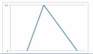
• Uses the estimate values based on the 3 point estimates that we covered during the chapter on Interviewing. The Optimistic, Most Likely and Pessimistic values from the 3 point estimate will be used here 
• Use only 3 values 
• Is used to quantify risks for each of the WBS elements 

Remember WBS? WBS stands for Work Breakdown Structure. 

The following is a sample Triangular Distribution


Normal and Lognormal Distributions

Normal and Lognormal Distributions are very similar to one another. Their common features include: 

• They use Mean and Standard Deviation to quantify risks
• They gather the 3 point estimates, just like the Triangular distribution
• Standard Deviation is usually displayed using either the Normal or Lognormal distributions


The Normal distribution:
• Is shaped like a bell curve
• The peak of the bell is the Mean/Average 
• Is typically used for variables that cluster around the Mean value 
• Is used to show confidence level as well as variations 

The following is a sample Normal Distribution



A lognormal distribution uses any random value, and those values plot just like a normal distribution. The following is a sample lognormal distribution. As you can see, the shape is pretty similar to the bell-curve of the normal distribution but distinctly different in terms of the actual shape. 



Uniform Distributions

• Are considered to be the simplest form of distributions
• Have all values of the same length which signifies equal probability
• Require you to know the upper and lower limits (the range) in order to use it 
• Show scenarios where no obvious value is more likely to happen than the other

For ex: if you were to throw a dice that isn’t rigged in any way, the chances of either of the 6 numbers turning up are equal and hence you will show that using this distribution. 

The following is a sample uniform distribution



Cumulative Distributions

Cumulative Distributions can convert a set of data values into a distribution that can be analyzed. They are typically S shaped. A sample Cumulative Distribution would look as follows:



There are two other types of distributions that would come under the blanket of Continuous Distributions. Though the PMBOK does not cover it, our chapter wouldn’t be complete if I don’t mention at least the definition of these two distributions. 

Exponential Distributions

The exponential distribution is used to represent the time between the arrival of random events that occur continuously and independently at an average rate

Gamma Distribution 

The Gamma distribution models the amount of time it would take for certain events to occur if the event occurs randomly with an average time between the events. Typically, gamma distributions are used to display waiting times. 

Trivia: 

Exponential and Gamma are not part of PMBOK or the PMI RMP Exam Syllabus

Before we wrap up this chapter on continuous distributions, let me reiterate that covering all possible details reg. each of these distributions is beyond the scope of the RMP exam and so I did not do it. If you have the time or the personal interest you can search Wikipedia or pick up a book on probability distributions to learn more about that. 


Lastly, if you know or rather remember whatever we have covered here, that should be more than sufficient from the PMI RMP Exam perspective. 


Prev: Introduction to Probability Distributions

Next: Discrete Distributions