Quantitative risk analysis is generally performed on risks that have been prioritized by using the qualitative risk analysis. However, depending upon the experience of the team and their familiarity with the risk, it is possible to skip the qualitative risk analysis and, after the risk identification, move directly to the quantitative risk analysis. The quantitative risk analysis has three major goals:
• Assess the probabilities of achieving specific project objectives
• Quantify the effect of the risks on the overall project objectives
• Prioritize risks by their contributions to the overall project risk
The image below explains the process more clearly.
Input to Quantitative Analysis
All the items that are input for the qualitative risk analysis are also input for the quantitative risk analysis. In addition, the quantitative risk analysis generally requires more information than its qualitative counterpart. The list of inputs for this process are:
• Risk register - The key input items from the risk register are the following:
o List of identified risksTo analyze the effect of risks on the project objectives, you need to know the project schedule and the project cost. These can be found in the cost management plan and schedule management plan. Also, the approaches taken by these plans can affect quantitative risk analysis.
o Priority list of risks if the qualitative risk analysis was performed
o Risks with categories assigned to them
o Management plans - To perform quantitative risk analysis, you must look at the risk management plan, cost management plan, and schedule management plan. To generate the output of the quantitative risk analysis, you need the following elements of the risk management plan:
Budgeting
Definitions of probabilities and impacts
Probability and impact matrix
Risk categories
Risk timing and scheduling
• Organizational process assets - The following organizational process assets might be useful in the quantitative analysis:
o Information on previously performed similar projects
o Studies performed by risk specialists on similar projects
o Proprietary risk databases or risk databases available from the industry
Tools and Techniques for Quantitative Analysis
The quantitative risk analysis can be looked upon as a two-step process; gathering and representing the data, and analyzing and modeling the data. Accordingly, all the techniques fall into two categories: data gathering and representation techniques, such as interviewing, probability distributions, and expert judgment; and analysis and modeling techniques, such as sensitivity analysis, EMV analysis, decision tree analysis, and modeling and simulation. We shall be covering them one by one in the list below:
Interviewing - This technique is used to collect the data for assessing the probabilities of achieving specific project objectives. You are looking for results such as: We have a 70% probability of finishing the project within the schedule desired by the customer. Or: We have a 60% probability of finishing the project within the budget of Rs. 100,000. The goal is to determine the scale of probabilities for a given objective; for example, there is a 20% probability that the project will cost Rs. 50,000, a 60% probability that it will cost Rs. 100,000, and a 20% probability that it will cost Rs. 150,000.
The data is collected by interviewing relevant stakeholders and subject matter experts. Most commonly, you will be exploring the optimistic (best case), pessimistic (worst case), and most likely scenarios for a given objective.
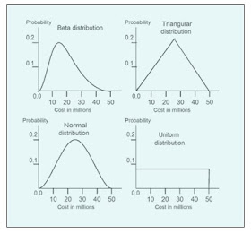
Probability distributions - After you have collected the data on meeting the project objectives, you can present it in a probability distribution for each objective under study. Note that a distribution represents uncertainty, and uncertainty represents risk. For example, if you know for sure the project will cost Rs. 25 lakhs, there will be no distribution because it is only one data point. Distribution comes into the picture when you have several possible values with a probability assigned to each value. There are distributions of different shapes in which the data can be presented.
Look at the picture above. This example is for the cost objective. The X axis represents the cost, and the Y axis represents the corresponding probability that the project will be completed within that cost.
The beta distribution and the triangular distribution are the most frequently used distributions. The other commonly used distributions that could be suitable under given circumstances are normal distribution and uniform distribution. The uniform distribution is used when all the values of an objective have the same chance of being true.
Sensitivity analysis - This is a technique used to determine which risk has the greatest impact on the project. You study the impact of one uncertain element on a project objective by keeping all other uncertain elements fixed at their baseline values. You can repeat this analysis for several objectives, one at a time. You can also repeat this study for several uncertain elements (creating risks), one element at a time. This way, you can see the impact of each element (or risk) on the overall project separate from other elements (or risks).
Expected monetary value analysis - The expected monetary value (EMV) analysis is used to calculate the expected value of an outcome when different possible scenarios exist for different values of the outcome with some probabilities assigned to them. The goal here is to calculate the expected final result of a probabilistic situation. EMV is calculated by multiplying the value of each possible outcome by the probability of its occurrence and adding the results. For example, if there is 60% probability that an opportunity will earn you Rs. 1,000 and a 40% probability that it will only earn you Rs. 500, the EMV is calculated as follows:
EMV = 0.60×1000 + 0.40×500 = 600 + 200= 800
So the EMV in this case is Rs. 800. When you are using opportunities and threats in the same calculation, you should express EMV for an opportunity as a positive value and EMV for a threat as a negative value. For example, if there is a 60% chance that you will benefit from a risk by Rs. 1,000 and a 40% probability that you will lose Rs. 500 as a result of this risk, the EMV is calculated as follows:
EMV = 0.60×1000 - 0.40×500 = 600 – 200 = 400
Therefore, the EMV in this case is Rs. 400.
The concept of EMV can be presented in a decision-making technique, such as a decision tree analysis.
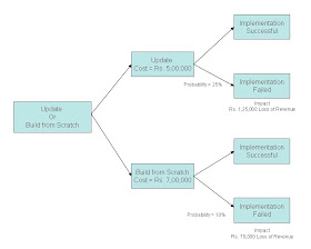
Decision tree analysis - This technique uses the decision tree diagram to choose from different available options; each option is represented by a branch of the tree. This technique is used when there are multiple possible outcomes with different threats or opportunities with certain probabilities assigned to them. EMV analysis is done along each branch, which helps to make a decision about which option to choose.
Look at the image below. It is a simple decision tree.
The decision tree diagram above depicts two options: updating an existing product or building a new product from scratch. The initial cost for the update option is Rs. 500,000, whereas the initial cost for the build-from-scratch option is Rs. 700,000. However, the probability for failure is 25% for the update option, compared to 10% for the build-from-scratch option, and the impact from failure for case 1 is Rs. 1.25 lakhs whereas for the other it is only Rs. 70,000. In such a situation, the build from scratch may be chosen because, even though it costs more, the chances of failure as well as losses in case of a failure are lower than the update option.
Modeling and simulation - A model is a set of rules to describe how something works; it takes input and makes predictions as output. The rules might include formulas and functions based on facts, assumptions, or both. A simulation is any analytical method used to imitate a real-life system. Simulations in risk analysis are created using the Monte Carlo technique, which is named after the city of Monte Carlo; known for its casinos that present games of chance based on random behavior. Monte Carlo simulation models take random input iteratively to generate output for certain quantities as predictions. This technique is used in several disciplines, such as physics and biology, in addition to project management. In risk analysis, the input is taken randomly from a probability distribution, and the output for impact on the project objectives is predicted. The name “Monte Carlo” refers to the random behavior of the input.
Expert judgment - In quantitative risk analysis, expert judgment can be used to validate the collected risk data and the analysis used for the project at hand.
Output of the Quantitative Risk Analysis: Updated Risk Register
As with the Qualitative Analysis, the output of this process too is the updates to the Risk Register. The updates include:
• Probabilistic analysis of the project - This includes the estimates of the project schedule and cost with a confidence level attached to each estimate. Confidence level is expressed in percentage form, such as 95%, and it represents how certain you are about the estimate. You can compare these estimates to the stakeholders’ risk tolerances to see whether the project is within the acceptable limits.
• Probability of achieving the project objectives - Factoring in project risks, you can estimate the probability of meeting project objectives, such as cost and schedule, set forth by the current project plan. For example, the likelihood of completing the project within the current budget plan of Rs. 2 lakhs is 70%.
• Prioritized list of risks - Risks are prioritized according to the threats they pose or the opportunities they offer. Risks with greater threats (or opportunities) are higher on the list. The goal is to prioritize the response plan efforts to eliminate (or minimize) the impact of the threats and capitalize on the opportunities. The priorities are determined based on the total effect of each risk to the overall project objectives.
• Trends in the results - By repeating the analysis several times and examining the results, you might recognize a trend for specific risks. That trend might suggest further analysis or a specific risk response. In finding the trend, you can also take a look at the historical information on project cost, quality, schedule, and performance.
Prev: Performing Qualitative Analysis
Next: Planning Risk Response


No comments:
Post a Comment